Alternating Background Colour

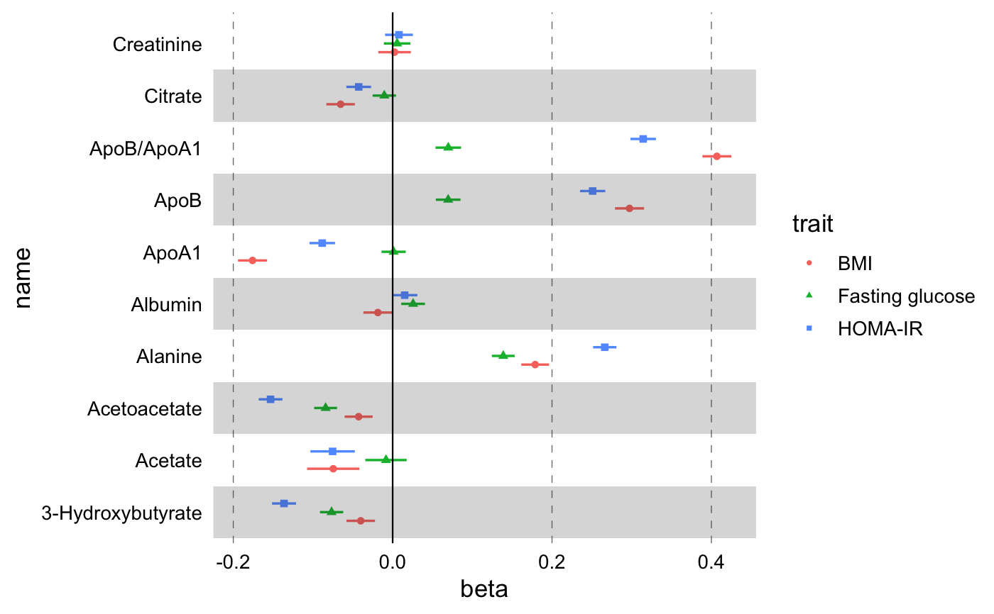
Add alternating background color along the y-axis. The geom takes default aesthetics odd and even that receive color codes. The codes would preferably be in the 8-hex ARGB format to allow for transparency if the geom is meant to be used as visual background.

geom_stripes(
  mapping = NULL,
  data = NULL,
  stat = "identity",
  position = "identity",
  ...,
  show.legend = NA,
  inherit.aes = TRUE
)

Arguments

mapping	Set of aesthetic mappings created by aes() or aes_(). If specified and inherit.aes = TRUE (the default), it is combined with the default mapping at the top level of the plot. You must supply mapping if there is no plot mapping.
data	The data to be displayed in this layer. There are three options: If NULL, the default, the data is inherited from the plot data as specified in the call to ggplot(). A data.frame, or other object, will override the plot data. All objects will be fortified to produce a data frame. See fortify() for which variables will be created. A function will be called with a single argument, the plot data. The return value must be a data.frame, and will be used as the layer data. A function can be created from a formula (e.g. ~ head(.x, 10)).
stat	The statistical transformation to use on the data for this layer, as a string.
position	Position adjustment, either as a string, or the result of a call to a position adjustment function.
...	Other arguments passed on to layer(). These are often aesthetics, used to set an aesthetic to a fixed value, like colour = "red" or size = 3. They may also be parameters to the paired geom/stat.
show.legend	logical. Should this layer be included in the legends? NA, the default, includes if any aesthetics are mapped. FALSE never includes, and TRUE always includes. It can also be a named logical vector to finely select the aesthetics to display.
inherit.aes	If FALSE, overrides the default aesthetics, rather than combining with them. This is most useful for helper functions that define both data and aesthetics and shouldn't inherit behaviour from the default plot specification, e.g. borders().

Examples

library(ggplot2)
library(magrittr)
df <-
  # Use built-in demo dataset
  df_linear_associations %>%
    # Arrange by name in order to filter the first few biomarkers for more
    # than one studies
    dplyr::arrange(name) %>%
    # Estimate confidence intervals
    dplyr::mutate(
      xmin = beta - qnorm(1 - (1 - 0.95) / 2) * se,
      xmax = beta + qnorm(1 - (1 - 0.95) / 2) * se
    ) %>%
    # Select only first 30 rows (10 biomarkers)
    dplyr::filter(dplyr::row_number() <= 30) %>%
    # Add a logical variable for statistical significance
    dplyr::mutate(filled = pvalue < 0.001)

g <-
  ggplot(data = df, aes(x = beta, y = name)) +
  # And point+errorbars
  geom_effect(
    ggplot2::aes(
      xmin = xmin,
      xmax = xmax,
      colour = trait,
      shape = trait,
      filled = filled
    ),
    position = ggstance::position_dodgev(height = 0.5)
  )
print(g)

# Add custom theme, horizontal gray rectangles, vertical line to signify the
# NULL point, custom color palettes.
g <-
  g +
  # Add custom theme
  theme_forest() +
  # Add striped background
  geom_stripes(odd = "#33333333", even = "#00000000") +
  # Add vertical line at null point
  geom_vline(
    xintercept = 0,
    linetype = "solid",
    size = 0.4,
    colour = "black"
  )
print(g)