Exploratory Analysis

Fit multiple regression models in one go.

discovery_regression(
  df_long,
  model = c("lm", "glm", "coxph"),
  formula,
  key = key,
  predictor = predictor,
  verbose = FALSE
)

Arguments

df_long	a data frame in a long format that contains a key column with the names of the variables for which to estimate the measures of effect, e.g. Nightingale NMR biomarker names, a value column with the numeric values of the respective keys and other columns with the response and other variables to adjust for. Note: You may use tidyr::gather to collapse your data frame to key-value pairs; it is recommended to dplyr::select only the variables that you want to go into your model, in order to avoid memory overheads in case of large datasets.
model	a character, setting the type of model to fit on the input data frame. Must be one of 'lm', 'glm' or 'coxph', for linear, logistic and cox proportional hazards regression, respectively.
formula	a formula object. For the case of models 'lm' and 'glm' it must be an object of class stats::formula (or one that can be coerced to that class): a symbolic description of the model to be fitted. The details of model specification are given under ‘Details’ in the documentation of stats::formula. For the case of model 'coxph', the formula object must have the response on the left of a ~ operator, and the rest of the terms on the right. The response must be a survival object, as returned by the Surv function.
key	the name of the key variable.
predictor	the name of the variable for which (adjusted) univariate associations are estimated. This is stated here in order to individuate the predictor of interest over many, possible cofactors that are also present in formula.
verbose	logical (default FALSE). If TRUE it prints a message with the names of the predictor and outcome. This may come in handy when, for example, fitting multiple outcomes.

Value

A data frame with the following columns: a character variable with the same name as the key parameter and numeric variables estimate, se and pvalue with the values of the respective variables of the linear model. If predictor is factor, additional column term is returned indicating factor level of predictor

Examples

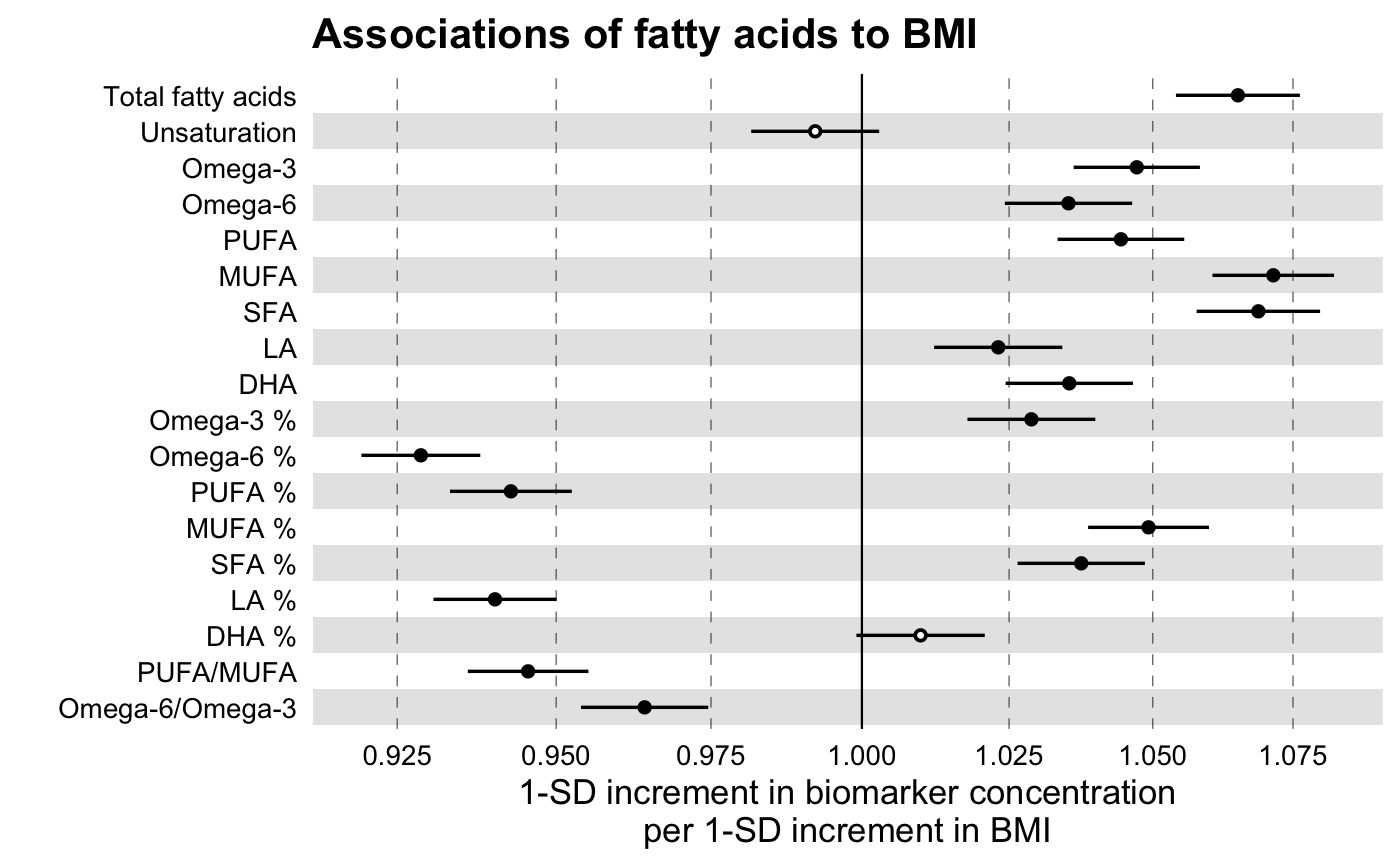
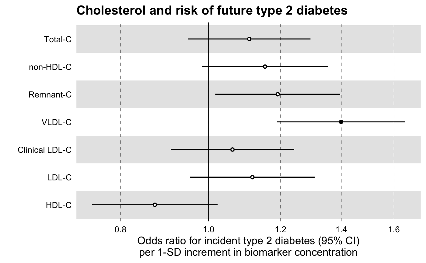
library(magrittr)

# Linear Regression Example

# We will use the simulated demo data that come with the package,
# ggforestplot::df_demo_metabolic_data

# Extract the names of the NMR biomarkers for discovery analysis
nmr_biomarkers <- dplyr::intersect(
  ggforestplot::df_NG_biomarker_metadata$machine_readable_name,
  colnames(df_demo_metabolic_data)
)

# Select only variables to be used for the model and collapse to a long
# format
df_long <-
  df_demo_metabolic_data %>%
  # Select only model variables
  dplyr::select(tidyselect::all_of(nmr_biomarkers), gender, BMI) %>%
  # Log-transform and scale biomarkers
  dplyr::mutate_at(
    .vars = dplyr::vars(tidyselect::all_of(nmr_biomarkers)),
    .funs = ~ .x %>% log1p() %>% scale() %>% as.numeric()
  ) %>%
  # Collapse to a long format
  tidyr::gather(
    key = machine_readable_name,
    value = biomarkervalue,
    tidyselect::all_of(nmr_biomarkers)
  )

df_assoc_per_biomarker <-
  discovery_regression(
    df_long = df_long,
    model = "lm",
    formula =
      formula(
        biomarkervalue ~ BMI + factor(gender)
      ),
    key = machine_readable_name,
    predictor = BMI
  )

# Filter Nightingale metadata data frame for biomarkers of interest
df_grouping <-
  ggforestplot::df_NG_biomarker_metadata %>%
  dplyr::filter(group %in% "Fatty acids")

# Join the association data frame with the group data above
df <-
  df_assoc_per_biomarker %>%
  # use right_join, with df_grouping on the right, to preserve the order of
  # biomarkers it specifies.
  dplyr::right_join(., df_grouping, by = "machine_readable_name")

# Draw a forestplot of the results
ggforestplot::forestplot(
  df = df,
  name = name,
  estimate = estimate,
  se = se,
  pvalue = pvalue,
  psignif = 0.001,
  xlab = "1-SD increment in biomarker concentration
per 1-SD increment in BMI",
  title = "Associations of fatty acids to BMI",
  logodds = TRUE
)

# Logistic Regression Example

# Extract names of relevant NMR biomarkers
nmr_biomarkers <- dplyr::intersect(
  ggforestplot::df_NG_biomarker_metadata$machine_readable_name,
  colnames(df_demo_metabolic_data)
)

# Select only variables to be used for the model and
# collapse to a long format
df_long <-
  df_demo_metabolic_data %>%
  # Select only model variables (avoid memory overhead)
  dplyr::select(
    tidyselect::all_of(nmr_biomarkers),
    gender,
    incident_diabetes,
    BMI,
    baseline_age
  ) %>%
  dplyr::mutate_at(
    .vars = dplyr::vars(tidyselect::all_of(nmr_biomarkers)),
    .funs = ~ .x %>% log1p() %>% scale() %>% as.numeric()
  ) %>%
  # Collapse to a long format
  tidyr::gather(
    key = machine_readable_name,
    value = biomarkervalue,
    tidyselect::all_of(nmr_biomarkers)
  )

df_assoc_per_biomarker_gender <-
  discovery_regression(
    df_long = df_long,
    model = "glm",
    formula =
      formula(
        incident_diabetes ~ biomarkervalue + factor(gender) + BMI + baseline_age
      ),
    key = machine_readable_name,
    predictor = biomarkervalue
  )

# Filter Nightingale metadata data frame for biomarkers of interest
df_grouping <-
  ggforestplot::df_NG_biomarker_metadata %>%
  dplyr::filter(
    group %in% "Cholesterol",
    !(machine_readable_name %in% c("HDL2_C", "HDL3_C"))
  )

# Join the association data frame with the group data above
df <-
  df_assoc_per_biomarker_gender %>%
  # use right_join, with df_grouping on the right, to preserve the order of
  # biomarkers it specifies.
  dplyr::right_join(., df_grouping, by = "machine_readable_name")

# Draw a forestplot of the results
ggforestplot::forestplot(
  df = df,
  name = name,
  estimate = estimate,
  se = se,
  pvalue = pvalue,
  psignif = 0.001,
  xlab = "Odds ratio for incident type 2 diabetes (95% CI)
per 1-SD increment in biomarker concentration",
  title = "Cholesterol and risk of future type 2 diabetes",
  logodds = TRUE
)